Scientific Portfolio’s Investment Philosophy ANNEX Summary of Functionalities

Scientific Portfolio’s Investment Philosophy ANNEX Summary of FunctionalitiesUser Solution Guide | April 2023

1. Highlights of SP functionalities- Financial considerations

1.1 Data Management and holdings-based analysis

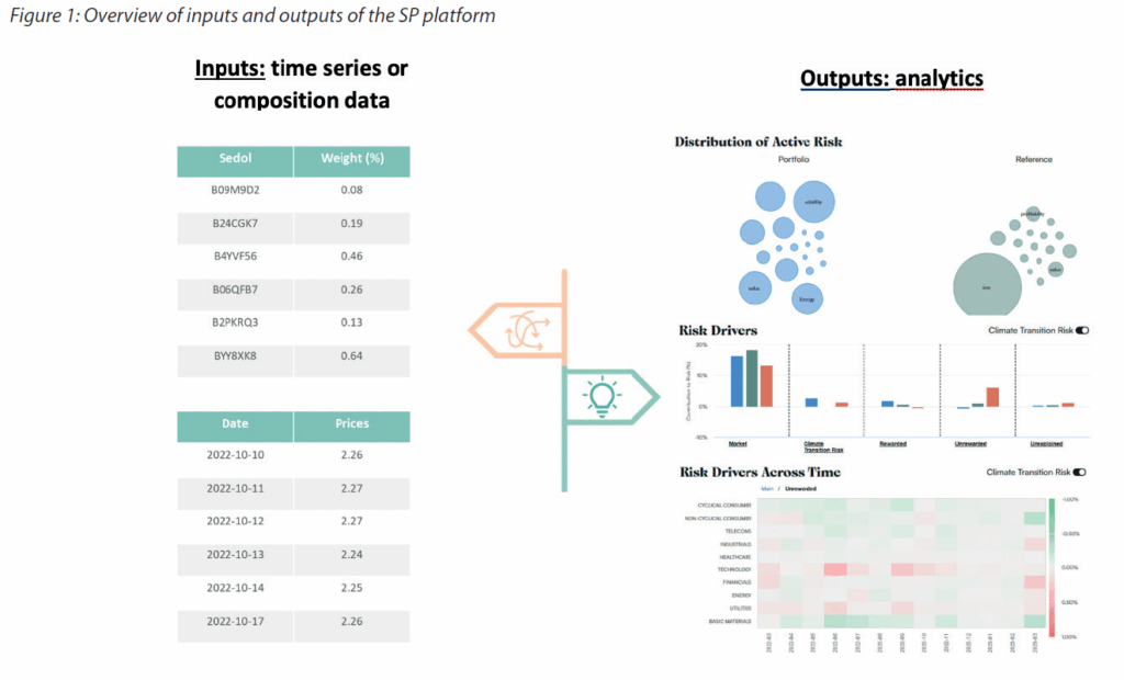
Easily upload your portfolio onto the Scientific Portfolio platform with a time series of returns or a stock-level composition. Use the holdings-based allocation to reveal concentrated positions or unintended sector or country biases at the aggregate portfolio level.

Data management is a core strength of the Scientific Portfolio (SP) platform, designed to streamline the process of uploading and editing portfolio data and enable users to easily compare a portfolio to a chosen reference and peer group. By simply uploading time series data or selecting from the set of available funds, ETFs or indices within the Scientific Portfolio database, users can create portfolios and gain access to actionable insights through quantitative risk analytics. Additionally, providing a portfolio’s stock-level composition will also unlock additional holdings-based analytics.

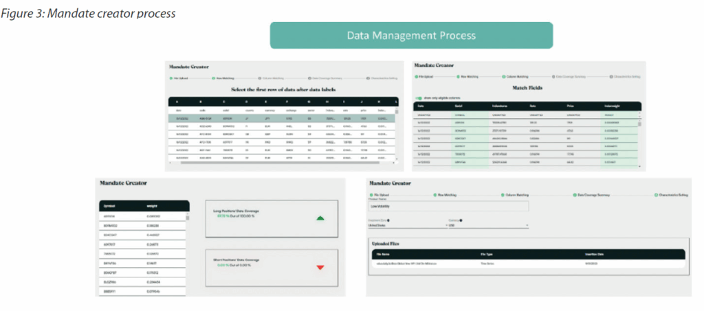
Thanks to a user-friendly interface, users can simply upload their portfolio composition or time-series data into a project. This process may be accomplished in a few simple steps, as demonstrated in Figure 2. We illustrate the data management process by uploading the composition of a portfolio. We begin by creating a new portfolio and defining a name, investment zone and currency as shown in Figure 2. To finalize the file upload, simply choose the format of data and drag the file onto the platform.

Upon successful upload, the ‘Mandate Creator’ is launched, providing guidance through a series of steps to complete the data management process. These steps include row matching, column matching, confirming the data coverage summary and naming the instrument. Figure 3 shows each step in detail.

Note that it is also possible to simply add items to a portfolio by searching the database with an ISIN code, Bloomberg ticker or Fund name. In the following example where stock-level holdings are known, we compare a portfolio comprised of two equally weighted funds from Developed Europe denominated in Euros to a reference. The reference is a market-cap weighted benchmark comprised of the 600 largest stocks in Europe.

Performance and Risk Overview

We begin with an overview comparison of the portfolio and reference shown in Figure 4.

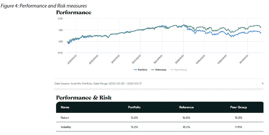
The portfolio has a lower annualized return over the period considered and exhibits a higher level of annualized volatility compared to the reference. Note that analysis can be conducted over a six month, one year, three year or five year period.

Sector, Country and Currency Allocations

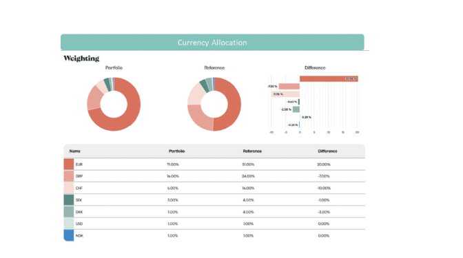
Holdings-Based Allocation shows the content of a portfolio as if it were a single fund, allowing for a clear view of capital allocation in terms of sectors, countries and currencies. Such an X-Ray view can reveal concentrated positions as well as highlight instances where there is little or no exposure. Note that knowledge of a portfolio’s composition is required to analyze a portfolio’s overall asset allocation.

The allocation of both the portfolio and reference is shown in Figure 5. We can quickly identify the specific sectors, countries and currencies where the greatest differences in allocation exist.

1.2 Risk-Adjusted Performance Analysis

Mitigate the backward-looking nature and sample dependence of the Sharpe ratio to assess whether your portfolio’s risk adjusted return is statistically significant
and therefore more likely to repeat out of sample.

The Sharpe ratio (SR) is a widely recognized metric that effectively captures the risk-reward profile of a portfolio. The SR measures the expected value of the return of an investment relative to the level of risk incurred. It therefore answers the question: to what extent has my financial performance compensated me for the risks that I have taken? However, the computation of SR is sample-dependent and is subject to estimation errors. To address this issue, we compute a confidence interval around our estimation. This approach enables us to determine the statistical significance of a portfolio’s SR, as well as whether a portfolio’s SR is significantly higher compared to the reference. The statistical significance provides assurance that the observation is not a one-off occurrence and is likely to be consistent out-of-sample. This is important for investors who wish to go beyond a backward-looking explanation and wish to identify forward-looking insights to take investment actions.

Below, in Figure 6, we compare the SR of a Dividend Income fund compared to a cap-weighted index representative of the 500 largest US public companies over a 3-year period and a 6-month period.

Over the course of 3 years, the SR is similar, and the confidence interval for the SR is also consistent. Comparing over 6 months, the Dividend Income fund has a higher SR; however, the size of the confidence interval exceeds the estimated SR value, which indicates the SR is not statistically significant. There is therefore a large degree of uncertainty associated with the SR, resulting in a lack of confidence that this superior performance will persist in the long term.

1.3 Factor-based Risk Analysis

Get a unique “risk identification card” of your portfolio and uncover unwanted exposures (betas). Determine your beta to academic (rewarded) equity factors and sector-based (unrewarded) factors to assess the long-term risk-adjusted return potential of your portfolio.

Factor Profile

Using only time series data, we generate a Factor Profile that shows a portfolio’s sensitivity (or beta) to a set of risk factors. The Scientific Portfolio platform computes a portfolio’s exposure to seventeen risk factors, which are divided into two categories: seven rewarded risk factors (including the Market risk factor) which are considered as persistent drivers of long-term returns, and ten unrewarded risk factors which are linked to sectors. These seventeen exposures to risk factors serve to collectively represent a risk identification card of the portfolio. The Factor Profile allows for an intuitive and comprehensive understanding of the systematic equity risks affecting the portfolio. In particular, it is relatively easy to identify whether a long-only portfolio is, beyond the obvious Market exposure, primarily exposed to rewarded factors or unrewarded factors, and hence, whether its strategic allocation contains sources of long-term risk-adjusted performance. This information is a crucial component in the decision-making process when deciding which actions to take to enhance a portfolio.

Factor Profiles of well-known indices

To build some intuition with respect to the Factor Profile, we examine four classic, broad-based cap-weighted indices in Figure 7. A cap-weighted index representative of the 500 largest US public companies (i.e., an S&P 500-like benchmark) is set as the reference.

The iShares S&P 500 and Russell 1000 ETFs display similar profiles, with minimal exposures to factors other than the Market. However, the iShares NASDAQ 100 and iShares Russell 2000 ETF display exposures to multiple factors beyond the Market. The NASDAQ 100 ETF is highly exposed to the Technology sector, while the Russell 2000 ETF, which mainly consists of smaller-cap funds, has a large exposure to the Size factor. As the Size factor tends to move together with cyclical sectors during different economic cycles, the Russell 2000 ETF also has a positive exposure to cyclical sectors such as Cyclical Consumer, Financials and Industrials (explained in more detail in Section 1.4).

Can you solely rely on a name?

The Factor Profile can also be a valuable tool for comparing a specific fund to a competitor. As an example, we present a comparison of the Factor Profile for two funds which are labeled as Value focused. One is shown as the portfolio and the other as the reference in Figure 8.

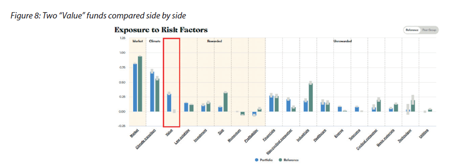
While both funds are allegedly Value focused, the reference has virtually no exposure to the Value risk factor, whereas the portfolio has a significantly positive exposure to it. Note that the Factor Profile makes it possible to immediately detect unusual patterns without any knowledge of the holdings. In this example, it alerts us to potential inconsistencies between the fund names and the portfolio’s risk exposures.

1.4. Sector Analysis

Examine your portfolio’s capital allocation across sectors. Then complement this knowledge with a risk-based view that uses the factor profile to identify relationships between sectors and rewarded factors and reveals all the risk exposures created by your capital allocation.

The Scientific Portfolio platform offers two perspectives on sector allocation (sectors are primarily derived from The Refinitive Business Classification (TRBC) Level 1 sectors).

The first perspective is the holdings-based sector allocation view, which shows how capital is distributed across a portfolio’s sectors. It is important to note that an understanding of a portfolio’s composition is necessary to analyze its sector allocation. While the holdings-based sector allocation view allows for a detection of some concentrated exposures (e.g., a portfolio allocated to only one or two sectors can be easily spotted), it is insufficient on its own to understand how a portfolio’s risks are spread once capital allocation spans several sectors. Therefore, it should be complemented with a risk-based view.

The second perspective is the risk-based view, which uses the factor profile and sensitivities to sector linked unrewarded factors to detect any unintended exposures that may arise when constructing a portfolio.

Viewing sector allocation through a risk-based lens offers two distinct advantages not available through the holdings-based allocation perspective. First, it allows for the identification of relationships between sectors, which facilitates an understanding of the relative pattern of movements between sector returns. Second, it can uncover exposures to associated rewarded factors when taking a long position in a particular sector.

To illustrate the difference between the holdings-based allocation view and risk-based view, we review a Healthcare fund as an example. The holdings-based sector allocation and risk-based view are represented in Figure 9.

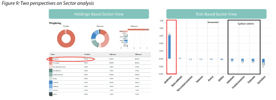
The sector allocation of a Healthcare (Defensive) fund is expected to be focused on the Healthcare sector by definition; however, as demonstrated by its Factor Profile, in addition to a strong positive exposure to Healthcare, there are some negative exposures to Industrials, Cyclical Consumer and Financials (Cyclical sectors), despite no explicit capital allocation to these sectors. The risk view therefore helps highlight the relationships between sectors, an insight that is not possible to identify from a holdings-based allocation view alone. These observations are in line with the typical behavior of Defensive and Cyclical sectors which tend to exhibit opposing patterns during different stages of the economic cycle. This relationship is captured by the risk factor exposures, demonstrating the natural divide between defensive and cyclical sectors.

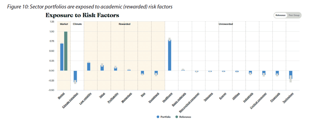
An additional insight that can be derived from the risk view is the resulting exposures to rewarded factors that arise from a strategic allocation. A detailed examination of the full Factor Profile reveals that there are additional considerations beyond simply having a large risk exposure to a particular sector when going long that sector. Figure 10 shows that the strategic allocation in this case has led to negative exposures to the Size and Investment factors. By identifying these short exposures to rewarded factors, it is possible to tilt the portfolio to address them, thereby potentially reducing portfolio risk and enhancing the risk-adjusted return over the long-term.

1.5. Risk Decomposition

Decompose your portfolio’s absolute and relative risk into individual and non-overlapping factor risk contributions, thus understanding the historical sources of your portfolio’s realized volatility and tracking error. Identify the key risk drivers across time to gain an insight into how risk manifests itself.

The total risk figure is only the beginning of the story because as explained in Section 1.2, statistical estimates are sample-dependent and may not be robust out of sample. Two funds with the same overall portfolio risk could have very different sources of risk, and therefore, behave very differently across various market regimes. By decomposing risk, we can delve deeper into the headline figure, identify the main drivers of risk over a period of time, build a more informed view on out-of-sample persistence, and understand how to control risk.

To decompose risk, the Factor Profile is interpreted by the Scientific Portfolio risk model and translated into seventeen non-overlapping systematic risk contributions and one idiosyncratic risk contribution, which can be further decomposed across instruments and time, providing different granular views of how risk manifests itself. Summing all contributions (for both rewarded and unrewarded factors)together will yield the exact volatility of a portfolio, resulting in a precise and transparent way to measure the origins of risk.

First, we review the drivers of two funds with similar levels of volatility.

While the total volatility is similar for each fund, Figure 11 shows the primary sources of risk are quite different, whether we look at risk contributions linked to the rewarded academic factors or the unrewarded sector-linked factors.

Translation of Factor Exposures to Risk Contributions

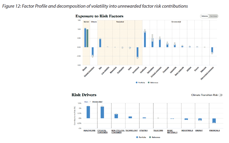
It is important to note that a material contribution to risk signifies a material exposure, but the converse is not always true, particularly over shorter time periods. This highlights the possibility that a risk exposure may not have had sufficient time to fully manifest itself and contribute to realized risk. The Factor Profile in Figure 12 shows that the Portfolio has a significant exposure to Technology; however, the contributions to risk from Technology are minimal.

It should also be emphasized that the sign of a risk contribution may not always align with its corresponding exposure owing to the inter-factor correlations. For instance, positive exposures to two factors that are negatively correlated will generally lead to offsetting risk contributions. On the other hand, two factors that are negatively correlated but have different directions of exposures will generally have risk contributions that are in the same direction, such as the Cyclical Consumer and Non-Cyclical Consumer risk factors in Figure 12.

We demonstrate the effect on risk of these correlations by introducing a Non-Cyclical Consumer fund into the portfolio. The addition of the Non-Cyclical Consumer fund increases the exposure to Non-Cyclical Consumer. Subsequently, in Figure 13, a comparison of the original portfolio against the modified portfolio reveals that both the contribution to risk from the Non-Cyclical Consumer sector and the overall risk is reduced.

It is noteworthy that the Non-Cyclical Consumer (Consumer Staples) fund has the effect of mitigating risk from the Non-Cyclical Consumer risk factor contribution. Despite being counterintuitive, the inclusion of the Non-Cyclical Consumer fund diminishes the overall risk of the portfolio by raising the exposure to a risk factor that exhibits negative correlation with the existing cyclical risk factors in the portfolio. In other words, the addition of a more defensive fund has counterbalanced the risk pattern of the more cyclical funds in the portfolio.

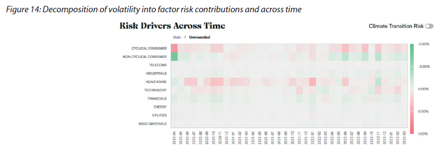
An aspect of risk that is frequently overlooked is the historical dimension, which views risk across time. It is often the case that the majority of total risk is attributed to a few short periods of time. Risk tends to appear in bursts, which can be identified on our platform, as shown in Figure 14.

1.6. Diversification Analysis

Assess and manage your portfolio’s diversification using both traditional, holdings-based analytics and a complementary risk-based diversification measure. Determine whether your portfolio is well “risk-diversified” and therefore associated with a more stable tracking error for risk budgeting purposes.

The Scientific Portfolio platform offers a comprehensive set of diversification analytics, enabling users to evaluate the diversification of a portfolio through both traditional, holdings-based metrics and advanced, risk factor-based methods.

To begin with, Effective Number (EN) of Stocks quantifies diversification by measuring the distribution of capital across instruments within a portfolio. It therefore accounts for the dominant effect of large weighted holdings compared to small-weighted holdings. On our platform, we provide the effective number of stocks, sectors, currencies, and countries. However, while EN metrics assess the concentration of a portfolio from a holdings perspective, they do not take risk into account. For instance, a portfolio holding a very large number of stocks may still be heavily concentrated, from a risk standpoint, into a given factor like Size, Low Risk, or Technology.

To address this limitation, we wish to introduce a risk-based EN measure. However, since our analytics are designed for long-only equity portfolios, the Market factor is expected to consistently be a very large risk contributor, giving an impression of concentration. It is therefore necessary to correct for this natural bias by performing our analysis on the active (i.e., relative to the regional market capitalization weighted benchmark) performance and active risk of the portfolio. Accordingly, we introduce a risk-based measure of diversification called Active Risk Diversification (ARD). Using only historical returns data, the Scientific Portfolio risk model decomposes systematic active risk (i.e., the portion of a portfolio’s active risk explained by the systematic risk factors) into seventeen individual factor-based active risk contributions. Treating each risk contribution as the weight of a separate “constituent asset” in the portfolio allows for a measurement of the historical degree to which active risks have been spread across all rewarded and unrewarded risk factors. Therefore, ARD represents the effective number of active risk contributions, with a low figure indicating that active risk is concentrated in a few factors and a high figure indicating a spread across multiple risk factors. If active risk were equally distributed across all risk factors (this theoretical allocation is often called a “risk parity” approach), the value of ARD would be seventeen.

Academic literature has placed a significant emphasis on diversifying across risk factors as it can provide several benefits, notably an increased stability in overall risk. In the context of active risk, the natural risk measure through which this stability may be observed is the tracking error. A recent Scientific Portfolio1 publication finds evidence to support this concept and demonstrates that ARD can facilitate risk budgeting by identifying funds likely to experience a more stable tracking error due to diversification. Directing attention towards portfolios which are diversified in terms of risk increases the likelihood of being able to manage the level of risk being budgeted.

To illustrate these concepts, we analyze the diversification of two Small-Cap portfolios shown in Figure 15.

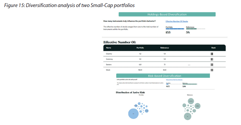
From a holdings perspective, the portfolio appears to be well diversified with a high EN of stocks equal to 153. However, from a risk point of view, the active risk within the portfolio is heavily concentrated into the Size risk factor, leaving the remaining risk factors to only make a small contribution to total active risk. While capital is clearly well-allocated across the portfolio constituents, the resultant risk is concentrated due to the similarities (a large portion of the constituents are small-cap equities) of the underlying stocks. Conversely, the Reference, despite having a lower ENS, has managed to effectively diversify its active risk across multiple factors (generally leading to a more stable TE historically than the portfolio).

1.7. Extreme Risks

Add another dimension to your portfolio’s risk analysis by incorporating downside tail risk. Robustly estimate your portfolio’s expected loss during a hypothetical worst week of the year and identify its origins and drivers thanks to our risk model and long-term risk factors that we use to simulate historical returns (addressing the issue of sparsity in extreme returns).

While volatility is the most popular measure for risk, extreme risk metrics are important for providing an insight into downside tail risk. The Scientific Portfolio platform uses two key metrics, Maximum Drawdown and Conditional Value at Risk (CVaR), to measure extreme risk.

Maximum Drawdown

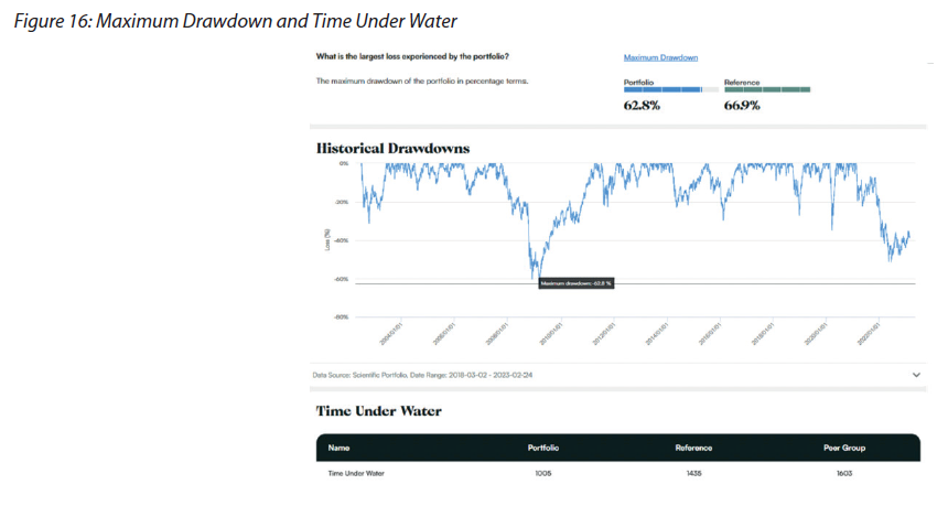
Maximum Drawdown (MDD) is a commonly used metric that quantifies the maximum observed loss experienced by a portfolio. It is defined as the largest peak-to-trough decline in the historic value of a portfolio, providing insight into the worst-case scenario of an investment. However, when evaluating the MDD of a portfolio which includes instruments which have different lengths of historical returns data available, the construction process can become challenging. For instance, a fund with historical data that includes the 2008 financial crisis is likely to have a higher MDD than a more recently established fund that does not have realized returns for that specific period. To address this limitation, we leverage the Scientific Portfolio risk model to simulate returns for periods when realized returns are not available. This approach ensures that MDD is comparable across different portfolios, regardless of data availability. While Maximum Drawdown explains the size of the largest loss, it does not provide an indication of the time it took to recover the loss. To gain insight into the recovery period, the metric ‘Time Under Water’ is often used. Time Under Water gives an indication of whether an investment had a shorter or longer recovery period to get back to the level before the loss.

Figure 16 shows the MDD and time under water for two funds with similar levels of volatility. The reference exhibits a higher MDD as well as a longer time to recovery.

Conditional Value at Risk

Conditional Value at Risk (CVaR), also known as “expected shortfall”, is a risk metric that offers a more conservative assessment of portfolio risk than volatility. It measures the expected loss that can be incurred a severe scenario (we aim for a level of severity no lower than the “worst week of a given year”, in other words a 2% CVaR), providing insight into potential downside tail risk. Therefore, if an investor wishes to budget risk based on large losses, CVaR would be a more suitable metric than volatility.

Like any measure of extreme risk, it is challenging to precisely estimate CVaR because it is based on a small fraction of the available returns, making it less stable and more sensitive to the period chosen than volatility. For this reason, popular techniques simulate more data using historical distributions. However, these techniques often rely on the inaccurate assumption that portfolio returns are normally distributed, which can lead to underestimating the amplitude of extreme events. To address this issue, Scientific Portfolio takes a two-step approach for the evaluation of a portfolio’s CVaR. First, we use the portfolio’s risk exposures with respect to the long-term factors of the Scientific Portfolio risk model to make realistic simulations of a portfolio’s returns over the last 15 years.

Second, we use this larger set of returns data and feed it into an analytical model suited for fat-tailed, non-normally distributed returns, making it possible to both estimate downside extreme risk (consistently with historical returns) and decompose it into contributions attributable to a portfolio’s exposures to risk factors. As an example, we review the CVaR of the funds shown in the previous section. Figure 17 shows that the portfolio has a slightly lower CVaR than the reference: on “the worst week of the year”, it could potentially lose 6.7% of its market value while the reference could lose 8.9%.

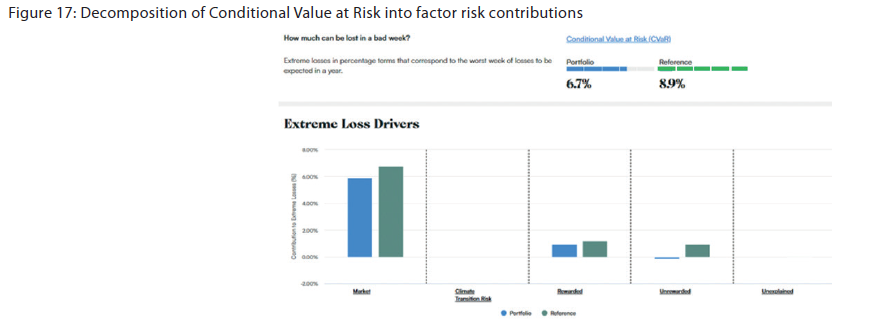
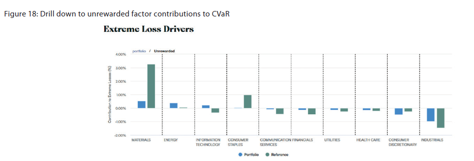
Drilling down to Unrewarded factor contributions in Figure 18 shows that one particular source of risk, the Materials sector, drives the contribution to extreme losses for the reference.

1.8. Macroeconomic sensitivities

Assess your portfolio’s exposure to macroeconomic factors and identify unintended or concentrated exposures to manage macroeconomic tilts.

In addition to rewarded and unrewarded equity fundamental risk factors, macroeconomic risk factors may also be used to explain a portfolio’s risk, although academic finance has not found any evidence of an equity risk premium associated with these factors. The macroeconomic factor exposure profile provides an understanding of how a portfolio is linearly exposed to various macroeconomic surprises (equities are forward-looking instruments so only genuinely new macroeconomic information may affect their price) relating to inflation, volatility, term spread, credit spread and short and long-term rates. The macroeconomic exposures (betas) are estimated after adjusting for the Market factor and therefore represent a macroeconomic sensitivity that is not already captured by portfolio’s natural exposure to the Market factor. Macro betas can be used to identify any unintended or concentrated exposures, making it possible to manage macro tilts. While exposures to macroeconomic risk factors may often be minimal, large movements in these factors can have a significant impact on a portfolio. As an example, we showcase the macroeconomic exposures of a fund with intuitive economic behavior: an Energy fund (compared to an S&P 500-like reference that has no macro betas by design as per above) in Figure 19.

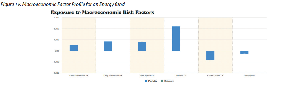
The Energy sector tends to be positively correlated with inflation and perform relatively well during periods of elevated inflation. This correlation can be attributed to the fact that the revenues of energy stocks are closely tied to energy prices, which are a key component of inflation indices.

2. Highlights of SP functionalities- ESG considerations

Our platform helps investors capture the double materiality of ESG investing, i.e., both ESG risk (see section 2.1 below) and ESG impact (see section 2.2).

2.1. Climate Transition (CT) Risk Analysis

Scientific Portfolio has developed a Climate Transition (CT) risk factor that allows investors to identify, measure and manage climate transition risk in a way that is similar to all other financial risks affecting a portfolio. Our approach is fully described in one of our recent research publications2. Our CT factor captures both the sectoral and intra-sectoral dimensions of transition risks by relying on a climate policy relevant sectors classification and on greenhouse gas emissions intensity. The implementation details are available on our platform.

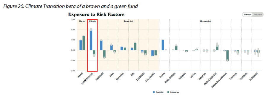
The CT risk factor is used to evaluate the level of exposure a portfolio has to climate transition. Long and short exposures to CT effectively represent market bets. A long exposure indicates a belief that brown members of a transition-sensitive sector will outperform their green counterparts while a short exposure bets that brown members of a transition-sensitive sector will underperform their green counterparts.

Using only time-series data, the CT exposure (beta) can determine whether the constituents of a portfolio are considered green or brown in terms of their climate transition efforts. To demonstrate that the CT beta indeed aligns with intuition, we review the exposure to CT for a portfolio of energy funds versus a clean energy reference. Intuitively, the energy portfolio will have a significant positive exposure while the clean energy fund will have a negative exposure to CT. The results, as depicted in Figure 20, confirm this expectation.

In Figure 21, we analyze how the exposure to CT translates into the CT contribution to risk.

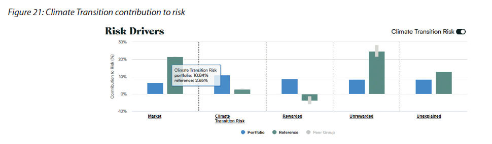
The CT contribution to risk shows the contribution of each risk factor to the overall climate transition risk of the portfolio. Our recent research findings are consistent with the financial literature and indicate that introducing the CT factor does not currently increase the overall explanatory power of our risk model. In other words, the CT risk is already explained by other more traditional factors, but it does provide another informative way to “slice the same overall risk pie”. As a result, the CT risk contribution overlaps with other factor risk contributions and therefore, when activated, transfers risk contributions away from other risk factors into the CT risk factor. In some cases, CT can explain a significant part of active risk. The energy portfolio has a risk contribution of 10.8% resulting from Climate Transition risk while the clean energy reference has a risk contribution of 2.7%, much lower as expected given the size of the respective CT betas.

To further demonstrate the actionable nature of our CT risk factor, we present an example in Figure 22 that depicts a portfolio consisting of multiple funds. The CT exposure is heavily influenced by a single fund, the Fidelity Select Energy Portfolio. We construct a modified version of the portfolio, excluding the aforementioned fund, and designate it as the reference portfolio.

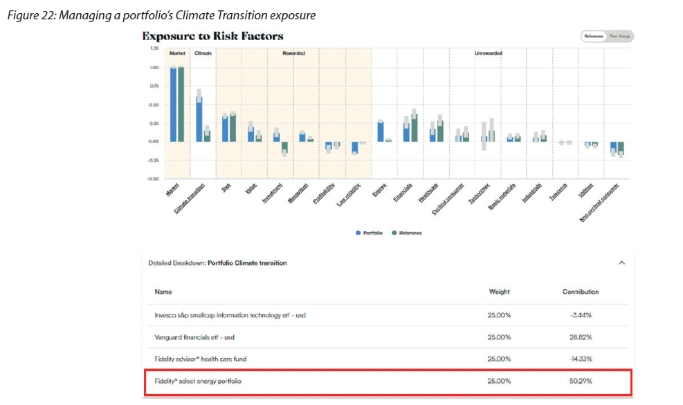
By removing the largest contributor and redistributing the weights evenly across the portfolio, the exposure to the CT factor is reduced to less than 15%, resulting in a risk contribution of 0.8%. However, there are other implications to removing the fund; specifically, while the intended goal of reducing exposure to CT is achieved, unintended consequences arise, such as a decrease in exposure to the Value and Investment risk factors. Assuming that exposure to these risk factors is desired, then the next step would be to either reconsider the removal of the fund with a material long CT exposure, or to find a replacement fund that has sufficient Value and Investment exposure without CT exposure.

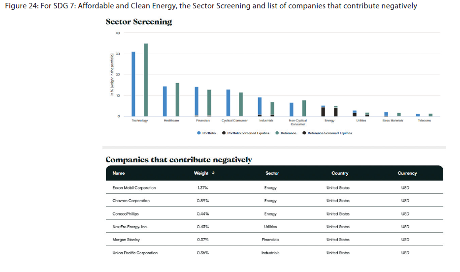
2.2. SDG-Aligned Impact Analysis via ESG Screening

Use our ESG screening tool to assess whether your portfolio is consistent with a consensus exclusion policy used by the largest asset owners in the world. Go beyond the consensus and use our proprietary screening policies to estimate the negative contributions (if any) of your portfolio to one or several of the United Nations’ Sustainable Development Goals (SDGs).

Scientific Portfolio’s ESG investment framework is based on a double materiality approach, with, on the one hand, the management of financial risks induced by ESG criteria (e.g., transition risks, see Section 2.1), and, on the other hand, the management of the impact of a portfolio on sustainable development. We view ESG screening as the first step in analysing the extra-financial impact of a portfolio and in building a more sustainable portfolio.

While mindful of the attempts made by some regulators to define what a « sustainable investment » is (see for instance Article 2 (17) of EU’s Sustainable Finance Disclosure Regulation), we propose to return to the historical origins of the concept of sustainable development to design a consistent and practical framework for sustainable investors.

The seminal 1987 Brundtland report provided a definition of sustainable development that is still in use today: a development that “[…] meets the needs of the present without compromising the ability of future generations to meet their own needs.” However, the academic literature indicates the concept was already known in the 18th century. Carl von Carlowitz, who oversaw the silver mining operations in Saxony (Germany) under the reign of King Frederick Augustus I, used the word “sustainability” in 1713 when he recommended stopping the overexploitation of forests, which he saw at the time as a risk on the wood supply chain. A few decades later, in the spring of 1789, Thomas Jefferson suggested to his friend Lafayette that he add an article specifically dedicated to the “rights of future generations” in what was to become (a few months later) the French Declaration of the Rights of Man and of the Citizen. Although there is evidence that Lafayette did submit the article it was not included in the final draft… Jefferson, who was the US ambassador in Paris at the time, clarified his views on the matter in a letter sent to James Madison a few months later:

“The question whether one generation of men has a right to bind another, seems never to have been started either on this or our side of the water. Yet it is a question of such consequences as not only to merit decision, but place also, among the fundamental principles of every government. […] I set out on this ground, which I suppose to be self evident, “that the earth belongs in usufruct to the living”: that the dead have neither powers nor rights over it […] Then no man can, by natural right, oblige the lands he occupied, or the persons who succeed him in that occupation, to the payment of debts contracted by him.” (6 September 1789)

While Carlowitz’ motivations were primarily economic and Jefferson’s were undoubtedly political and philosophical, both shared the idea that sustainability was, in their mind at least, first and foremost about protecting the world, not necessarily improving it.

The original and historical definition of sustainable development was therefore much closer to a do no harm (DNH) injunction, possibly a very strict one, than a call to action to do good and change the world (although there is, in principle, nothing wrong with attempting to do good!). The nature of the “harm” should be clarified in practice, and the United Nations’ 17 Sustainable Development Goals (SDGs) seem like a very useful tool to define the environmental and social goods that ought to be protected.

Given the DNH essence of the concept of sustainability, ESG screening and exclusion policies are a natural lever for ESG investors and are expected to play a central role in the design of sustainable investment portfolios. That’s why, the Scientific Portfolio platform uses screening policies (exclusion lists) to analyse the negative impacts (if any) of a portfolio on the United Nations’ 17 Sustainable Development Goals (SDGs). We have analyzed each SDG and its associated metrics (when relevant data is available) and produced a set of screening policies that align with each SDG.

In practice, our platform currently offers two pre-built ESG screening policies:

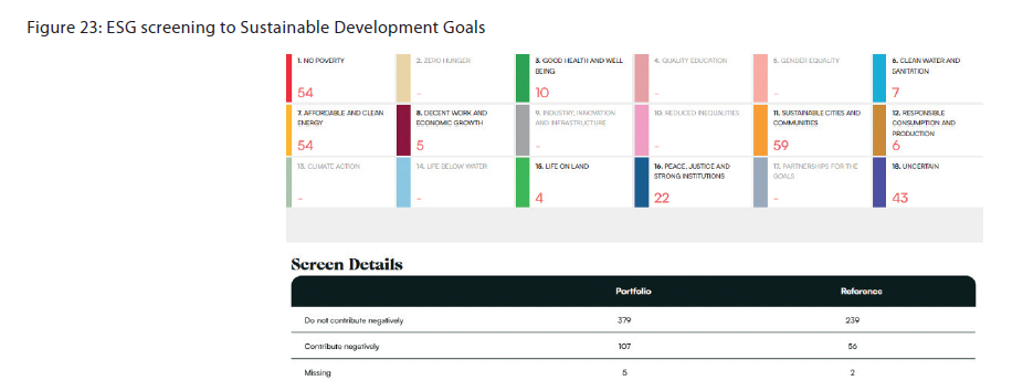
The Sustainable Development Goals Screen highlights any company whose behaviour and activities undermine the achievement of one or more of these goals.
The Consensus Screen is based on a set of criteria derived from an analysis of the exclusion policies of the 100 largest asset owners.

To illustrate the functionalities offered on our platform, we conduct a screening analysis on an S&P 500 ntracker (referred to as “Portfolio”) and an S&P500 ESG fund (referred to as “Reference”) to determine the number of companies in violation of one of the Sustainable Development Goals. The ESG screening in Figure 23 reveals that 107 stocks within the portfolio have a negative contribution to sustainable development, while the Reference only has 56.

We then apply a screen pertaining to SDG 7: Affordable and Clean Energy focused on the issue of Fossil Fuels. In total, Figure 24 reveals that the majority of companies within the Energy sector for both the Portfolio and Reference are found to have a negative impact. For full transparency, a list of companies that contribute negatively to the specific SDG is provided in the accompanying table.